Loading... ## 原理 ### Canny Canny 边缘检测是一种经典的图像边缘检测算法,于 1986 年由 John F. Canny 提出。它是一种多阶段的算法,主要包括高斯滤波、计算图像梯度、非极大值抑制、双阈值处理和边缘跟踪等步骤。Canny 边缘检测算法的主要思想是尽可能准确地找出图像中的边缘,并将其提取为像素点集合,以便后续的图像分析和处理。 ### CNN 卷积神经网络(CNN)是一类深度学习模型,主要用于图像识别、目标检测和语义分割等计算机视觉任务。CNN 的核心组件是卷积层、池化层和全连接层。通过卷积层提取图像的特征,通过池化层减少特征图的大小,最后通过全连接层将特征映射到输出类别。CNN 在图像处理领域取得了巨大成功,其主要优点包括参数共享、局部感知性和平移不变性等。 ### ResNet 残差网络(ResNet)是由 Kaiming He 等人于 2015 年提出的一种深度神经网络架构。ResNet 提出了残差模块的概念,通过引入跳跃连接(或称为快捷连接)来解决深度神经网络训练中的梯度消失和梯度爆炸问题。ResNet 的主要创新是使用残差块(Residual Block),这种块可以学习残差函数,从而在理论上允许网络层数增加时仍然保持良好的性能。ResNet 在 ImageNet 等大规模图像数据集上取得了令人瞩目的成绩,成为了深度学习领域的重要里程碑之一。 ## 环境 * TensorFlow * OpenCV * Python ## 实验 ### 提取数字图像 对于多手写数字识别来说,首先需要将图片中的多个数字提取为单个数字,方便后续的处理。 #### Canny 边缘检测 对于一张需要提取特征的图片,首先就要提取图像的边缘,一种常用的方法就是 Canny 算法进行边缘检测,这里使用 OpenCV 库来操作,当然,在操作之前,需要先将图片转为二值图来方便提取。 ```python gray_image = cv2.cvtColor(image, cv2.COLOR_BGR2GRAY) _, binary_image = cv2.threshold(gray_image, 127, 255, cv2.THRESH_BINARY) edges = cv2.Canny(binary_image, 50, 100) ``` #### 轮廓检测 在使用 Canny 算法提取边缘之后,我们就可以尝试提取数字的轮廓了,在 OpenCV 中提供了一个专门的方法 `cv2.findContours` 来提取边缘,对于一个数字来说,我们只需要最外侧的边缘即可,但是这样会遇到一些问题,某些封闭数字比如说数字 8 在某些情况下可能会被识别为多个部分,因为这个数字具有多个轮廓,为了避免这种情况,我采取的方式是在处理轮廓时,判断有没有出现在内部的轮廓,如果有则跳过。 ```python contours, _ = cv2.findContours(edges, cv2.RETR_EXTERNAL, cv2.CHAIN_APPROX_SIMPLE) recognized_rectangles = [(x, y, w, h) for x, y, w, h in map(cv2.boundingRect, contours)] contour_image = image.copy() for contour in contours: x, y, w, h = cv2.boundingRect(contour) overlapping = any( rx < x and rx + rw > x + w and ry < y and ry + rh > y + h for rx, ry, rw, rh in recognized_rectangles ) if not overlapping: square_image = image[y - 5:y + h + 10, x - 5:x + w + 10] cv2.rectangle(contour_image, (x - 5, y - 5), (x w + 10, y + h + 10), (0, 255, 0), 2) ``` #### 图片预处理 在提取出每一张数字图片后,我们还需要对图片进行预处理来符合模型输入的要求,对于模型来说,输入的图片的格式应当是 (28,28,1) 的大小,同时需要注意的是,MNIST 数据集中的图片均为黑底白字,所以我们也要处理为黑底白字,同时 MNIST 中每一张的图片虽然大小为 28 但是有效区域的大小只有 20。 ```python image = cv2.bitwise_not(image) height, width, _ = image.shape side_length = max(height, width) out_length = int(side_length * 1.4) square_image = np.zeros((out_length, out_length, 3), dtype=np.uint8) x_start = (out_length - width) // 2 y_start = (out_length - height) // 2 square_image[y_start:y_start + height, x_start:x_start + width] = image gray_image = cv2.cvtColor(square_image, cv2.COLOR_BGR2GRAY) image_data = cv2.resize(gray_image, (28, 28)) image_data_for_prediction = np.array(image_data).astype('float32') / 255.0 image_data_for_prediction = np.expand_dims(image_data_for_prediction, axis=-1) image_data_for_prediction = np.expand_dims(image_data_for_prediction, axis=0) ``` ### 构建 CNN 这里使用 TensorFlow 自带的模型构建器参考 ResNet 构建了一个 CNN 模型,首先定义残差学习单元,由于识别数字的任务较为简单,这里使用了较浅的 ResNet-18。 #### 定义残差学习单元 ```python def basic_block(input_tensor, filters, stride=1): x = layers.Conv2D(filters, 3, strides=stride, padding='same')(input_tensor) x = layers.BatchNormalization()(x) x = layers.ReLU()(x) x = layers.Conv2D(filters, 3, padding='same')(x) x = layers.BatchNormalization()(x) if stride != 1 or input_tensor.shape[-1] != filters: input_tensor = layers.Conv2D(filters, 1, strides=stride)(input_tensor) input_tensor = layers.BatchNormalization()(input_tensor) x = layers.add([x, input_tensor]) x = layers.ReLU()(x) return x ``` #### 定义 ResNet-18 模型 ```python def build_resnet18(input_shape, num_classes): inputs = layers.Input(shape=input_shape) x = layers.Conv2D(64, 7, strides=2, padding='same')(inputs) x = layers.BatchNormalization()(x) x = layers.ReLU()(x) x = layers.MaxPooling2D(3, strides=2, padding='same')(x) x = basic_block(x, 64) x = basic_block(x, 64) x = basic_block(x, 128, stride=2) x = basic_block(x, 128) x = basic_block(x, 256, stride=2) x = basic_block(x, 256) x = basic_block(x, 512, stride=2) x = basic_block(x, 512) x = layers.GlobalAveragePooling2D()(x) outputs = layers.Dense(num_classes, activation='softmax')(x) return models.Model(inputs, outputs) ``` ### 训练模型 先尝试使用 SGD 作为优化器,训练轮数采用 10 轮,并定义回调函数,在训练过程中保存效果最好的模型。 ```python def normal_train(): model = build_resnet18((28, 28, 1), 10) model.compile(optimizer=tf.keras.optimizers.SGD(learning_rate=0.01, decay=1e-6, momentum=0), loss=tf.keras.losses.CategoricalCrossentropy(), metrics=['accuracy']) checkpoint = ModelCheckpoint('./normal_trained_model.h5', monitor='val_accuracy', save_best_only=True, mode='max', verbose=1) res = model.fit(train_images, train_labels, batch_size=64, epochs=10, validation_data=(test_images, test_labels), callbacks=[checkpoint]) showimg(res.history) ``` #### 训练结果 通过图像可以看到,训练时的准确率较高,但是测试集上的准确率相对偏低,有一点过拟合的趋势,出现过拟合的原因可能是 MNIST 数据集样本过于简单。 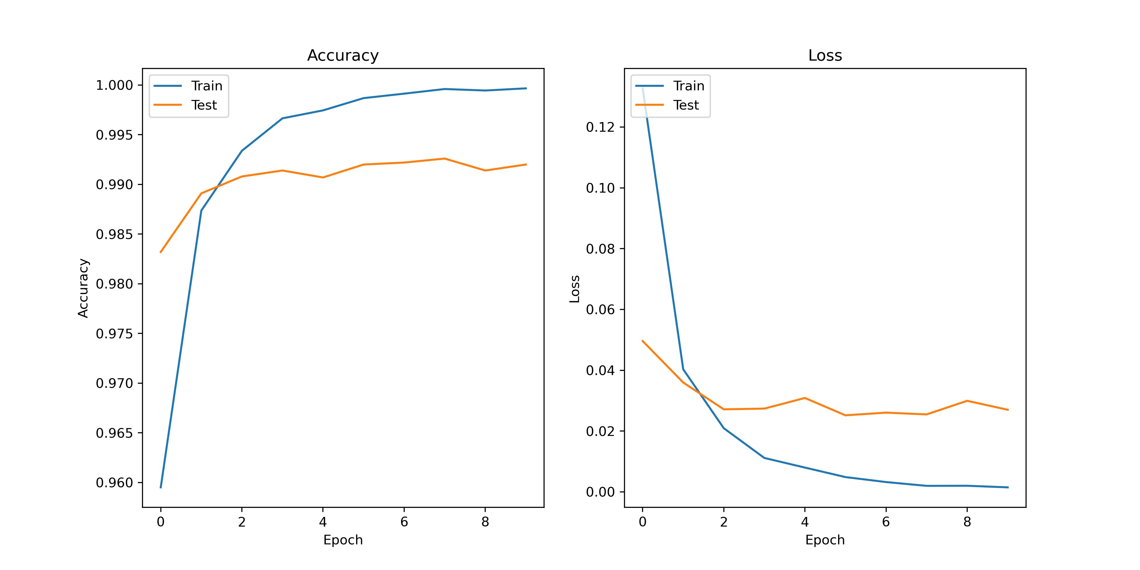 #### 图片预测 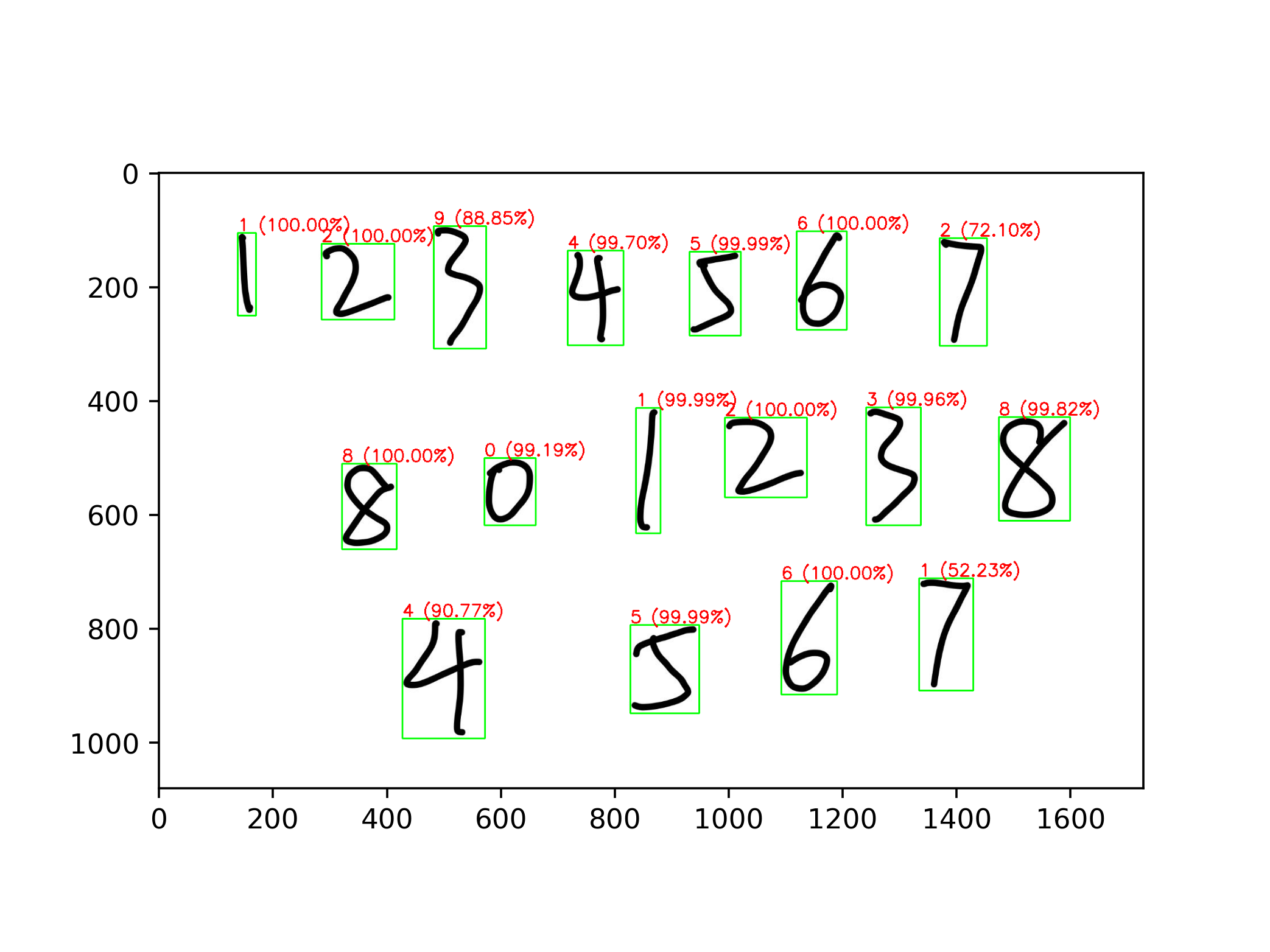 通过结果可以看到,有一些数字出现了识别错误的情况,甚至在错误的情况下给出了较高的可信度,经过分析可能有以下几个原因。 * MNIST 数据集中的数字是西文写法,有些数字的写法可能不同 * MNIST 数据集中的样本过少,特征太明显导致鲁棒性不强 * 图片预处理出现了问题 经过排查之后,第三个原因是不存在的,所以总结之后的原因就是样本数据太少,所以我们要重新训练模型。 ### 优化训练 #### 数据增强 数据增强是一种非常常见的手法,通过对原数据集进行不同程度的处理,比如拉伸,缩放,翻转等等,变相增加数据量的大小,这里使用 TensorFlow 自带的数据增强器进行操作,因为是数字图像,翻转后的数字是没有意义的,所以这里不进行翻转。 ```python datagen = ImageDataGenerator( rotation_range=20, width_shift_range=0.1, height_shift_range=0.1, zoom_range=0.1, horizontal_flip=False, vertical_flip=False ) ``` #### 更换优化器 原先使用的是 SGD 作为优化器,同样的,这个优化器也会导致一些问题的出现,比如出现局部最优解的情况,这里我们将优化器换为 Adam,它是一种自适应学习率的优化器,可以适配大部分情况,不过需要调整更多的超参数,设置学习率为 0.001。 ```python def optimize_train(): model = build_resnet18((28, 28, 1), 10) datagen = ImageDataGenerator( rotation_range=20, width_shift_range=0.1, height_shift_range=0.1, zoom_range=0.1, horizontal_flip=False, vertical_flip=False ) model.compile(optimizer=tf.keras.optimizers.Adam(learning_rate=0.001), loss=tf.keras.losses.CategoricalCrossentropy(), metrics=['accuracy']) checkpoint = ModelCheckpoint('./optimize_trained_model.h5', monitor='val_accuracy', save_best_only=True, mode='max', verbose=1) res = model.fit(datagen.flow(train_images, train_labels, batch_size=64), epochs=10, validation_data=(test_images, test_labels), callbacks=[checkpoint]) showimg(res.history) ``` #### 训练结果 可以看到,再采取数据增强后,整体的曲线质量更高了。 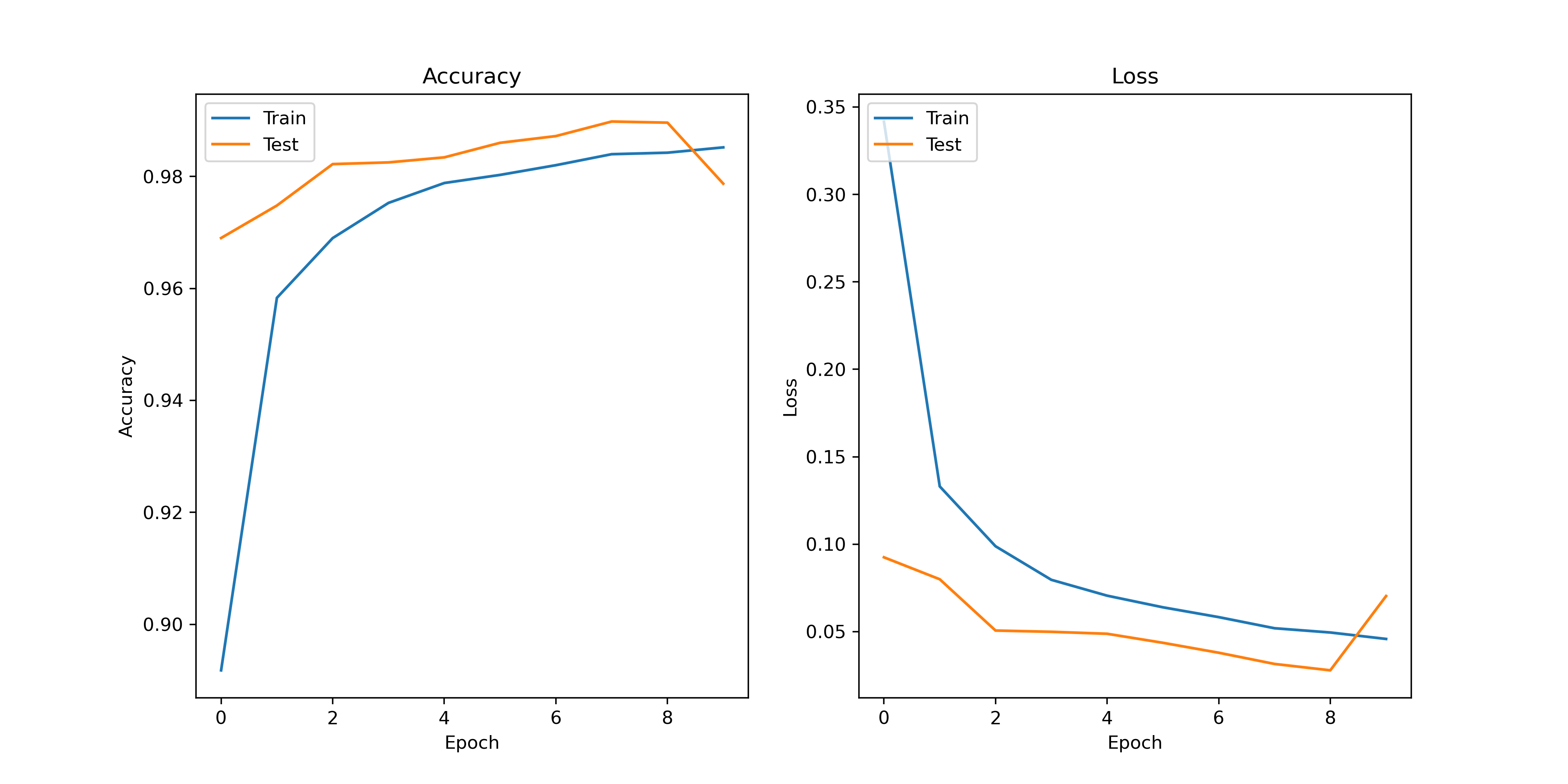 #### 图片预测  通过结果可以看到,进行优化后,整体准确率得到了提高。 ## 源代码 模型训练 <div class="panel panel-default collapse-panel box-shadow-wrap-lg"><div class="panel-heading panel-collapse" data-toggle="collapse" data-target="#collapse-c222b48b4384d7ffed2778413543dbf24" aria-expanded="true"><div class="accordion-toggle"><span style="">train.py</span> <i class="pull-right fontello icon-fw fontello-angle-right"></i> </div> </div> <div class="panel-body collapse-panel-body"> <div id="collapse-c222b48b4384d7ffed2778413543dbf24" class="collapse collapse-content"><p></p> ```python import tensorflow as tf from matplotlib import pyplot as plt from tensorflow.keras import layers, models from tensorflow.keras.datasets import mnist, fashion_mnist from tensorflow.keras.utils import to_categorical from tensorflow.keras.callbacks import ModelCheckpoint from tensorflow.keras.preprocessing.image import ImageDataGenerator # 加载MNIST数据集 (train_images, train_labels), (test_images, test_labels) = mnist.load_data() # 数据预处理 train_images = train_images.reshape((60000, 28, 28, 1)).astype('float32') / 255 test_images = test_images.reshape((10000, 28, 28, 1)).astype('float32') / 255 train_labels = to_categorical(train_labels) test_labels = to_categorical(test_labels) def basic_block(input_tensor, filters, stride=1): x = layers.Conv2D(filters, 3, strides=stride, padding='same')(input_tensor) x = layers.BatchNormalization()(x) x = layers.ReLU()(x) x = layers.Conv2D(filters, 3, padding='same')(x) x = layers.BatchNormalization()(x) if stride != 1 or input_tensor.shape[-1] != filters: input_tensor = layers.Conv2D(filters, 1, strides=stride)(input_tensor) input_tensor = layers.BatchNormalization()(input_tensor) x = layers.add([x, input_tensor]) x = layers.ReLU()(x) return x def build_resnet18(input_shape, num_classes): inputs = layers.Input(shape=input_shape) x = layers.Conv2D(64, 7, strides=2, padding='same')(inputs) x = layers.BatchNormalization()(x) x = layers.ReLU()(x) x = layers.MaxPooling2D(3, strides=2, padding='same')(x) x = basic_block(x, 64) x = basic_block(x, 64) x = basic_block(x, 128, stride=2) x = basic_block(x, 128) x = basic_block(x, 256, stride=2) x = basic_block(x, 256) x = basic_block(x, 512, stride=2) x = basic_block(x, 512) x = layers.GlobalAveragePooling2D()(x) outputs = layers.Dense(num_classes, activation='softmax')(x) return models.Model(inputs, outputs) # def build_lenet(input_shape, num_classes): # inputs = layers.Input(shape=input_shape) # # x = layers.Conv2D(32, (3, 3), activation='relu')(inputs) # x = layers.MaxPooling2D((2, 2))(x) # # x = layers.Conv2D(64, (3, 3), activation='relu')(x) # x = layers.MaxPooling2D((2, 2))(x) # # x = layers.Conv2D(64, (3, 3), activation='relu')(x) # # x = layers.Flatten()(x) # # x = layers.Dense(64, activation='relu')(x) # # outputs = layers.Dense(num_classes, activation='softmax')(x) # return models.Model(inputs, outputs) def normal_train(): model = build_resnet18((28, 28, 1), 10) # 编译模型 model.compile(optimizer=tf.keras.optimizers.SGD(learning_rate=0.01, decay=1e-6, momentum=0), loss=tf.keras.losses.CategoricalCrossentropy(), metrics=['accuracy']) checkpoint = ModelCheckpoint('./normal_trained_model.h5', monitor='val_accuracy', save_best_only=True, mode='max', verbose=1) # 训练模型并保存性能最好的模型 res = model.fit(train_images, train_labels, batch_size=64, epochs=10, validation_data=(test_images, test_labels), callbacks=[checkpoint]) showimg(res.history) def optimize_train(): model = build_resnet18((28, 28, 1), 10) # 数据增强 datagen = ImageDataGenerator( rotation_range=20, # 旋转角度范围 width_shift_range=0.1, # 宽度偏移范围 height_shift_range=0.1, # 高度偏移范围 zoom_range=0.1, # 缩放范围 horizontal_flip=False, # 不进行水平翻转 vertical_flip=False ) # 编译模型 model.compile(optimizer=tf.keras.optimizers.Adam(learning_rate=0.001), loss=tf.keras.losses.CategoricalCrossentropy(), metrics=['accuracy']) checkpoint = ModelCheckpoint('./optimize_trained_model.h5', monitor='val_accuracy', save_best_only=True, mode='max', verbose=1) # 训练模型并保存性能最好的模型 res = model.fit(datagen.flow(train_images, train_labels, batch_size=64), epochs=10, validation_data=(test_images, test_labels), callbacks=[checkpoint]) showimg(res.history) def showimg(history): # 绘制训练和验证准确率 plt.figure(figsize=(12, 6), dpi=326) plt.subplot(1, 2, 1) plt.plot(history['accuracy']) plt.plot(history['val_accuracy']) plt.title('Accuracy') plt.xlabel('Epoch') plt.ylabel('Accuracy') plt.legend(['Train', 'Test'], loc='upper left') # 绘制训练和验证损失值 plt.subplot(1, 2, 2) plt.plot(history['loss']) plt.plot(history['val_loss']) plt.title('Loss') plt.xlabel('Epoch') plt.ylabel('Loss') plt.legend(['Train', 'Test'], loc='upper left') # 显示图像 plt.show() ``` <p></p></div></div></div> 图片预测 <div class="panel panel-default collapse-panel box-shadow-wrap-lg"><div class="panel-heading panel-collapse" data-toggle="collapse" data-target="#collapse-15d55c96df1eb8b84b812103ef1b1a6796" aria-expanded="true"><div class="accordion-toggle"><span style="">predict.py</span> <i class="pull-right fontello icon-fw fontello-angle-right"></i> </div> </div> <div class="panel-body collapse-panel-body"> <div id="collapse-15d55c96df1eb8b84b812103ef1b1a6796" class="collapse collapse-content"><p></p> ```python import matplotlib.pyplot as plt import tensorflow as tf import numpy as np import cv2 def load_model(path): # 加载已训练好的手写数字识别模型 model = tf.keras.models.load_model(path) return model def predict_one(image, model): # 颜色反转为黑底白字 image = cv2.bitwise_not(image) # 获取图像的高度和宽度 height, width, _ = image.shape # 计算正方形的大小(取较大的那个维度作为边长) side_length = max(height, width) out_length = int(side_length * 1.4) # 创建一个黑色底的正方形图像 square_image = np.zeros((out_length, out_length, 3), dtype=np.uint8) # 计算粘贴的区域坐标 x_start = (out_length - width) // 2 y_start = (out_length - height) // 2 # 在正方形图像上粘贴原图像 square_image[y_start:y_start + height, x_start:x_start + width] = image # 将图像大小设为28*28并转换为灰度图像 gray_image = cv2.cvtColor(square_image, cv2.COLOR_BGR2GRAY) image_data = cv2.resize(gray_image, (28, 28)) # 将图像数据转为模型输入所需的格式 image_data_for_prediction = np.array(image_data).astype('float32') / 255.0 image_data_for_prediction = np.expand_dims(image_data_for_prediction, axis=-1) image_data_for_prediction = np.expand_dims(image_data_for_prediction, axis=0) # 使用模型进行预测 prediction = model.predict(image_data_for_prediction) prediction_label = np.argmax(prediction) prediction_confidence = np.max(prediction) # 返回结果 return prediction_label, prediction_confidence def find_counter(image): # 将图像转换为灰度图 gray_image = cv2.cvtColor(image, cv2.COLOR_BGR2GRAY) # 将灰度图转换为二值图 _, binary_image = cv2.threshold(gray_image, 127, 255, cv2.THRESH_BINARY) # 使用Canny边缘检测 edges = cv2.Canny(gray_image, 50, 100) # 查找轮廓 contours, _ = cv2.findContours(edges, cv2.RETR_EXTERNAL, cv2.CHAIN_APPROX_SIMPLE) return contours def predict_img(img_path, model_path): # 加载本地模型 model = load_model(model_path) # 读取一张原始图像图像 image = cv2.imread(img_path) contours = find_counter(image) # 保存所有的轮廓边界框的列表 recognized_rectangles = [(x, y, w, h) for x, y, w, h in map(cv2.boundingRect, contours)] # 在原始图像上绘制轮廓及正方形 contour_image = image.copy() b, g, r = cv2.split(contour_image) contour_image = cv2.merge([r, g, b]) for contour in contours: # 计算轮廓的边界框 x, y, w, h = cv2.boundingRect(contour) overlapping = any( rx < x and rx + rw > x + w and ry < y and ry + rh > y + h for rx, ry, rw, rh in recognized_rectangles ) if not overlapping: # 提取其中一张数字图片 square_image = image[y - 2:y + h + 4, x - 2:x + w + 4] # 将图片加入模型获取预测结果 prediction_label, prediction_confidence = predict_one(square_image, model) # 在原始图像上绘制轮廓同时添加结果 cv2.rectangle(contour_image, (x - 2, y - 2), (x + w + 4, y + h + 4), (0, 255, 0), 2) text = f"{prediction_label} ({prediction_confidence * 100:.2f}%)" cv2.putText(contour_image, text, (x + 2, y + 20), cv2.FONT_HERSHEY_SIMPLEX, 1.0, (255, 0, 0), 2) # 显示结果 plt.figure(dpi=326) plt.imshow(contour_image) plt.show() ``` <p></p></div></div></div> © 允许规范转载 打赏 赞赏作者 微信 赞

2 条评论
我抄了
你过关